As data clouds continue to become the de facto choice for data warehousing needs, a pattern has emerged over the past several years of transitioning from ETL to ELT. This pattern allows data teams to effectively transform data and monitor performance by moving the data transformation process directly within the data warehouse. Snowflake has been at the core of this transition since its inception. Especially with data transformation solutions like Coalesce enabling organizations with granular control over the data modeling process, it’s no surprise data teams continue to adopt an ELT process on Snowflake.
However, with this shift to running transformations on Snowflake comes an added workload on your virtual data warehouse(s) that can easily start to increase your bill. The good news is that Snowflake provides multiple avenues for optimizing your data transformation workloads to achieve optimal performance without sacrificing your budget.
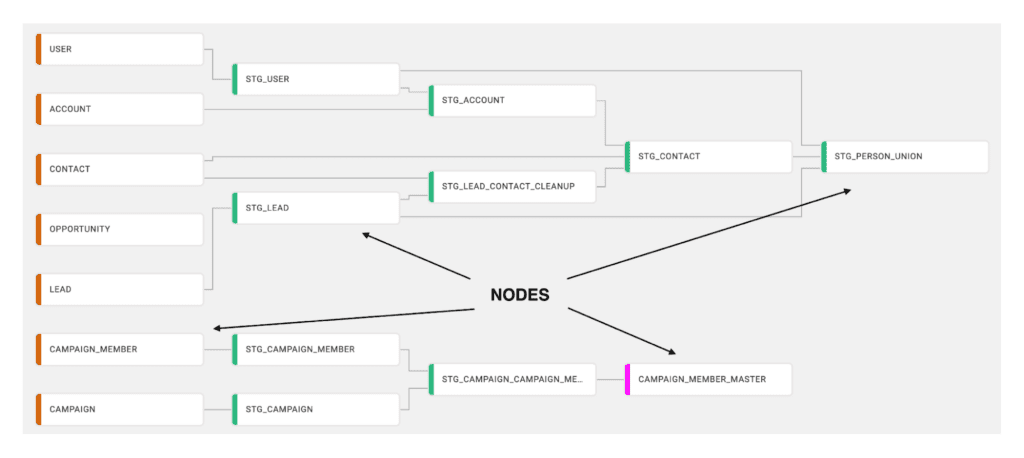
While exploring the cost optimization techniques in this article, I’ll be using Coalesce, a data transformation solution built exclusively for Snowflake, to demonstrate how these considerations can be implemented within your data transformation process. While these techniques can be applied using other data transformation solutions, whether homegrown or off-the-shelf, Coalesce makes implementing these optimizations seamless. Coalesce uses the term node to represent the creation and transformation of any database object within your data pipeline.
Don’t be afraid of views
When it comes to data transformation, a popular area for immediate cost optimization is evaluating how your Snowflake objects are materialized. The most common Snowflake objects used within data transformation are tables and views. While it is easy to default to building all objects in Snowflake as tables, it can be advantageous to evaluate using views for certain transformations, in order to optimize your Snowflake consumption.
When to use a view over a table
When determining whether to use a table or a view, a major item to explore is where in the DAG (directed acyclic graph) the specific node you are evaluating is located. If you are unfamiliar with DAGs, you can think of them as a pipeline that executes steps (nodes) in a specific order.
If the transformation is taking place early on (upstream) in your DAG, such as a staging node, and its primary purpose is to transform data for other downstream nodes, this is likely a good candidate to materialize as a view. There are three primary reasons a view may be a better choice than a table in this situation.
First, because this node is unlikely to be heavily queried (and probably should not be), creating this node as a view allows for users to save Snowflake compute for larger, more business-critical tables that will be heavily queried. By identifying nodes in your DAG that are not heavily queried and are primarily used as intermediate pass-throughs to transform data, you can give these nodes significant consideration for materializing as a view rather than a table.
Second, although briefly touched on already, it is important to note that Snowflake can build a view node faster than a table node. This is important because as your DAG continues to grow over time, the compute that can be saved by materializing dozens or hundreds of nodes as views can help save a significant amount of Snowflake compute, translating to larger cost savings.
Finally, while storage is often a fraction of the price of compute in Snowflake, by materializing nodes as views, you will not actually be storing data anywhere, thus alleviating any unnecessary storage cost.
While we’ve just made several arguments for changing nodes from tables to views, there are multiple advantages to using tables over views. The primary advantage is the query performance benefit obtained by allowing Snowflake to store and micro-partition data as a table. Tables can also be built relatively quickly if they are smaller and don’t contain complex logic. However, there are times where a node needs to be materialized as a table for query performance, but is taking a long time to run due to varying factors. In this case, consider the next strategy.
Consider incremental builds over full truncation
Within data modeling, it’s not uncommon for a fact or other business-critical table to contain a significant amount of ever-growing data. Additionally, it is not unusual for these same tables to be full truncations (delete all data and reload everything) every time they are updated.
For example, let’s say a business has a fact table containing 200 million records of order data at the beginning of the business day. On average, the business receives roughly 1 million orders per day. Let’s also assume that the business runs a final data transformation process at the end of each business day. If using a table truncation strategy, Snowflake will delete all current 200 million records, and rerun the query that obtains all 200 million of the previous records that were already in the table, plus the additional 1 million new order records—so the table will have 201 million records after the run.
As you can probably infer, depending on the complexity of the logic and how wide the table is, this process may take Snowflake multiple minutes to complete. For tables that have a large, increasing volume of data and also need optimal query performance, using a table incremental strategy can save a significant amount of Snowflake compute usage.
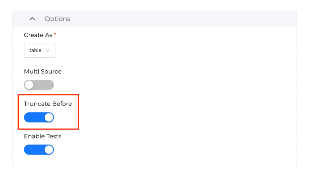
By using an incremental strategy, the data transformation process for the orders table we discussed would use an upsert, where only new or changed records will be processed, leaving all unchanged records in the table, avoiding the need to process them. In the case of the orders table, our process would now only have to process 1 million records per run, rather than 201 million. This change from truncation to incremental strategy can have a significant impact on your virtual data warehouse by lessening the amount of time the warehouse stays online to process data. Coalesce allows for this to be done through a simple toggle.
Use proper virtual warehouse sizes
Once you have determined how each node should be materialized and whether or not you should use an incremental strategy, another area of optimization worth exploring is the sizing of each virtual data warehouse. By controlling the sizes used by the data transformation process, you can gain additional cost optimization in Snowflake.
While a larger, more complex query may see increased performance when moving from an X-Small to Small warehouse in Snowflake, at some point the compute and optimization of that query is going to see negligible performance improvements as that query will not need any additional optimization or compute to run any faster. While this may vary depending on the data volume being processed, or the complexity of the query, it is important to note that query performance between a smaller warehouse and a larger warehouse may not be significant enough to justify the cost of the compute consumed.
Additionally, at the time of this writing, Snowflake’s auto-suspend configuration for a virtual data warehouse can be decreased down to 60 seconds. So if you run a query that takes 12 seconds to run, and do not run anything else on the warehouse, the warehouse will automatically suspend itself after 60 seconds elapse. This means that Snowflake will always charge you for at least 60 seconds of compute.
From an optimization perspective, if you are running queries that take less than 60 seconds to run and are variable in nature, you can eliminate wasted Snowflake consumption by adjusting to a smaller warehouse size. For example, let’s say you have an analyst that runs 30 simple ad hoc queries each hour on Snowflake. If each of these queries were run every other minute, you would be charged for 30 minutes of consumption (60 seconds of consumption X 30 queries), even if each query only took 15 seconds to run.
By evaluating the run time of queries on a warehouse, if a significant number of queries are taking less than 60 seconds to run, and lowering the warehouse size doesn’t make the queries run significantly longer, you can end up saving wasted Snowflake consumption, and therefore costs, by switching to a smaller virtual warehouse size.
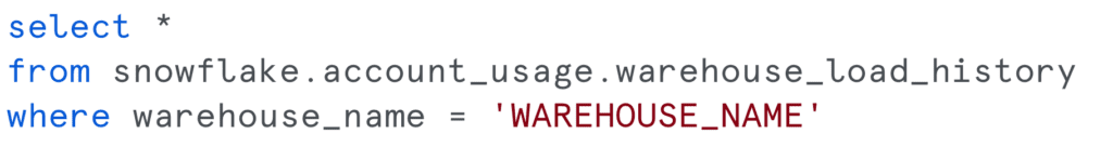
You can view the average load on your warehouse by viewing the warehouse load history table in Snowflake:
Consider breaking your CTEs into a pipeline
The last optimization technique we’ll discuss is breaking out your CTEs (common table expressions) into a DAG. By breaking each CTE into its own module or node, you can gain several advantages.
The first advantage is that when CTEs are split into their own nodes, you have more control over how those nodes are run. For example, let’s assume that a certain CTE query has five CTEs within it. Each CTE is feeding the next, and we want to get results from the fourth CTE even though we have five. While this result can be obtained within a CTE, it would typically require a coding refactor and—unless deleted from the SQL—also contain a fifth CTE, which at the very least adds bloat to your code.
By breaking each CTE out into its own node, you can control how each of those nodes are run and how they materialize, without having any excess code or wasted optimization. Additionally, when multiple CTEs are used within a data transformation project, it’s not uncommon for these CTEs to process similar, if not the same, data in different CTEs. For example, the result of one CTE may be to obtain all the order sales in the past 90 days, and the result of another CTE is to obtain any orders above $1,000 in the past 90 days.
In both scenarios, we would likely be processing the same data, specifically an orders table. This gives us the opportunity to create a fact table that only needs to be run once, and can be referenced by the downstream nodes. This helps save on consumption and makes the data modeling process significantly cleaner.
Not only is it possible to consolidate models and reuse them, but by creating our data modeling in a pipeline fashion, we create increased visibility and auditability into those nodes. When code is contained in a CTE, it can be painful and cumbersome to identify bugs or logic errors that may exist. When they are found, multiple parts, if not the full CTE, need to be run again to ensure the proper fix has been implemented.
By using a pipelining approach, we have much better visibility into what each node is doing. This allows us to quickly diagnose and easily identify issues within the DAG by isolating the errors to a specific node. Additionally, once a fix has been implemented, we can simply test that specific node instead of running everything upstream of the node and wasting Snowflake compute. Easier to debug and cheaper to run? A win for everyone.
Optimize your data transformations
Snowflake provides users with multiple avenues to optimize the data transformation process. By using a solution such as Coalesce, you can easily develop your data transformations in a way that optimizes your Snowflake consumption. Whether it’s breaking your CTEs into an easier-to-manage pipeline, or giving you the ability to convert a table to a view in just a few clicks, Coalesce gives you all the control needed to run best-practice Snowflake code and provide the best utilization for your Snowflake credits.